Alright, Nerds, it’s time to get serious.

I claimed that my last post was not going to be foundational, and then I went an wrote about pretty much everything which lies at the foundation of classical mechanics. Now it’s time I feel to distill all that down to the bare fundamentals, without the wrapper of a falling coin that my previous post provided.

So, let us, therefore, consider some object. It does not matter what that object is. It does not matter what shape it has. Its mass does not matter, nor does it does not matter what matter it’s made out of.

The only thing that matters about the object is that it exists. Somewhere.

Where?

As is often the case, \(x\) marks the spot.

Here, “\(x\)” represents some value that lies along a line called the “\(x\)-axis,” which is a number line that represents a pair of opposite directions in space. These could be any directions: north and south, to and fro, this way and that way, what-have-you. Traditionally, the \(x\)-axis is used to represent left and right, with right being the positive direction and left being negative. This means that like any good number line, the \(x\)-axis has three parts: a positive part, a negative part, and \(0\) directly between the two. That \(0\) is pretty important. It’s called the axis origin, and it serves as the reference point from which all values of \(x\) are counted.

So, our object’s position along the \(x\)-axis can be described with two pieces of information: a magnitude, which tells us how far away the object is from \(0\), and a direction that we represent with a \(+\) or \(-\) sign. In physics, quantities with magnitudes and directions are called vectors; specifically, all positions along our \(x\)-axis are position vectors.

Time for an example. Below I have drawn an \(x\)-axis, and along it, I have placed five objects that I’m calling \(A\), \(B\), \(C\), \(D\), and \(E\).

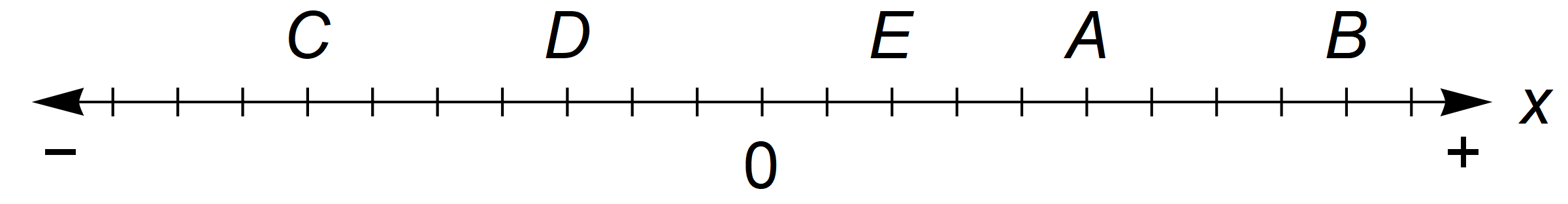
Their positions along the \(x\)-axis are \(x_A\), \(x_B\), \(x_C\), \(x_D\), and \(x_E\), respectively, and we can assign specific values with respect to \(0\) to each of them by counting the number of tick marks from the origin to the object in question and labeling that value with the appropriate sign indicating whether we are counting to the left or to the right: \begin{equation} \begin{aligned} & x_A = +5 \,\mathrm{ticks}, \\ & x_B = +9 \,\mathrm{ticks}, \\ & x_C = -7 \,\mathrm{ticks}, \\ & x_D = -3 \, \mathrm{ticks}, \\ & x_E = +2 \, \mathrm{ticks}. \end{aligned} \end{equation}

Note that we also stated what we counted—tick marks along our \(x\)-axis. Each one of those marks represents a single unit of whatever type of quantity we are dealing with—in this case, length. Since we never specified a length unit, each tick could represent one of any number of quantities, from the agate to the 丈 (zhàng) and anything in between, such as my favorite length: the Smoot. That said, from here on out, unless otherwise specified, I am sticking with the SI base length: the meter. Consequently, we should label our \(x\)-axis to reflect this fact:

\begin{equation} \begin{aligned} & x_A = +5 \,\mathrm{m}, \\ & x_B = +9 \,\mathrm{m}, \\ & x_C = -7 \,\mathrm{m}, \\ & x_D = -3 \, \mathrm{m}, \\ & x_E = +2 \, \mathrm{m}. \end{aligned} \end{equation}

There you have it—complete descriptions of five different objects along our \(x\)-axis with respect to the axis origin. If I give you those values and specify the axis origin and orientation, then you and your trusty meterstick can easily find all five things.

But how will I tell you where the origin is? Say that it’s \(3\,\mathrm{m}\) to the right of \(D\)? What about \(2\,\mathrm{m}\) to the left of \(E\)? Or even \(5\,\mathrm{m}\) to the left of \(A\)? Why not just set it at \(A\)? That’d be simple:

So now we have a new \(x\)-axis, parallel to the original one and with the same length unit, but set up such that object \(A\) lies at the new axis’ origin. Therefore, I’m calling it the \(x^A\)-axis. But now we have to go through the tedious process of recounting tick marks to find the positions of our objects with respect to this new origin.

Or do we?

Not if you’re willing to do a little arithmetic! Notice that because we placed the origin of the \(x^A\)-axis at object \(A\), object \(A\)’s position along that new axis is by definition \(0\,\mathrm{m}\). Now, ask yourself, “what must I do to any value, such as \(x_A\), to make it zero?” Answer: subtract that value from itself. Doing so to \(x_A\) yields: \begin{equation} x_A^A = x_A - x_A = \left( +5\,\mathrm{m} \right) - \left( +5\,\mathrm{m} \right) = 0\,\mathrm{m}. \label{06112019ta} \end{equation}

If we make the same change to the \(x\) values of the other object positions, meaning we subtract \(x_A\) from each other object’s \(x\) value along the original \(x\)-axis, we similarly obtain their equivalents along the \(x^A\)-axis: \begin{equation} \begin{aligned} & x_B^A = x_B - x_A = ( +9 \,\mathrm{m} ) - ( +5 \, \mathrm{m} ) = +4 \, \mathrm{m}, \\[1ex] & x_C^A = x_C - x_A = ( -7 \,\mathrm{m} ) - ( +5 \, \mathrm{m} ) = -12 \, \mathrm{m}, \\[1ex] & x_D^A = x_D - x_A = ( -3 \, \mathrm{m} ) - ( +5 \, \mathrm{m} ) = -8 \, \mathrm{m}, \\[1ex] & x_E^A = x_E - x_A = ( +2 \, \mathrm{m} ) - ( +5 \, \mathrm{m} ) = -3 \, \mathrm{m}. \end{aligned} \label{06112019tbcde} \end{equation}

I encourage you to count ticks along the \(x^A\)-axis to verify that these values are correct. Also, note how this procedure automatically changed the sign of object \(E\)’s position in concordance with the fact that it is now on the other side of the axis origin.

Of course, there is no reason, beyond possible convenience, why we had to place the axis origin at the location of object \(A\). In fact, we could have placed it anywhere! As far as we know, space has no origin and any point is just as valid as any other. Therefore, we can assign the axis origin to any of our objects and use the subtraction procedure above to find the consequent positions of everything else. In the following table I’ve done just that—each column lists the five object positions in meters along the axis indicated in the top row. \begin{equation} \begin{array}{r|rrrrr} \left(\mathrm{m}\right) & x^A & x^B & x^C & x^D & x^E \\ \hline x_A & 0 & -4 & +12 & +8 & +3 \\ x_B & +4 & 0 & +16 & +12 & +7 \\ x_C & -12 & -16 & 0 & -4 & -9 \\ x_D & -8 & -12 & +4 & 0 & -5 \\ x_E & -3 & -7 & +9 & +5 & 0 \\ \end{array} \label{06102019xtable} \end{equation}

And here is a picture to go with it:

The * in \(x^*\) stands for \(A\), \(B\), \(C\), \(D\), or \(E\), depending on whether \(O^A\), \(O^B\), \(O^C\), \(O^D\), or \(O^E\) is being used as the axis origin.

Along this axis, I have plotted five different origins corresponding to the five different objects, and I am now using the letter \(O\) to represent these origins instead of the number \(0\). This is because each origin is only at \(0\,\mathrm{m}\) along its own axis—it’s not at \(0\,\mathrm{m}\) along any other axis. For example, the position of \(O^A\) is \(0\,\mathrm{m}\) along the \(x^A\)-axis, but it’s \(-4\,\mathrm{m}\) along the \(x^B\)-axis and \(+3\,\mathrm{m}\) along the \(x^E\)-axis, etc. Yes, this makes things a bit cluttered, but you can use the image to verify that table \eqref{06102019xtable} is correct. Just start at any one of the origins and count off tick marks to any one of the objects. The origin’s superscript letter corresponds to the superscript of the axis you are using across the top of table \eqref{06102019xtable}, and the object’s letter corresponds to the subscript of the position you are measuring down the table’s left.

But alas, things are cluttered, so let’s clean it up a bit. Below, I have drawn yet another axis. Or rather, I have redrawn the one from above but this time with only two different origins that I am calling \(O\) and \(O’\). As you will see, \(O\) is actually \(O^A\) from above, the origin of the \(x^A\)-axis, but since that superscript is a bit cumbersome and not necessary going forward, I’m dropping it. Therefore \(O\) is the origin of what is now simply called the \(x\)-axis. Similarly, \(O’\) is the origin of the \(x’\)-axis, and that’s one we’ve not seen before. Note that this origin does not correspond to any of the objects, because, once again, origin’s don’t have to—they can be anywhere!

As before, \(x^*\) stands for either \(x\) or \(x’\), depending on whether \(O\) or \(O’\) is used as the axis origin, respectively.

Now, what are the positions of the objects along the new \(x\)-axis? They are the same as they were before when we called it the \(x^A\)-axis, but again, we’re dropping the superscript: \begin{equation} \begin{aligned} x_A &= 0 \, \mathrm{m}, \\ x_B &= +4 \, \mathrm{m}, \\ x_C &= -12 \, \mathrm{m}, \\ x_D &= -8 \, \mathrm{m}, \\ x_E &= -3 \, \mathrm{m}. \end{aligned} \end{equation}

But what are the positions of the objects along the \(x’\)-axis? Well, as always, you can find them by counting tick marks, but instead, I am going to do it by using the transformation procedure worked out above: the value of any position along the \(x’\)-axis can be derived from its value along the \(x\)-axis by subtracting the value of \(O’\)’s position along the \(x\)-axis.

lol, wut?

“How can \(O’\) have a position along the \(x\)-axis? Isn’t it part of the \(x’\)-axis?”

It can, and it is.

Yes, \(O’\) is the origin of the \(x’\)-axis. But it’s also has a position along the \(x\)-axis. (Note that we actually discussed this above, concerning the origin \(O^A\), which again is now called \(O\).) As usual, this position is found by starting at \(O\) and counting tick marks until you reach \(O’\). Doing so above tells us that \(x_{O’} = -10\,\mathrm{m}\). Why isn’t it zero? Because zero is the value of \(O’\)’s position along the \(x’\)-axis, not the \(x\)-axis. In other words, even though \(x’_{O’} = 0\,\mathrm{m}\) by definition, in general \(x’_{O’} \ne x_{O’}\), which can therefore be something else. Similarly, \(O\) has a position along the \(x’\)-axis which isn’t zero even though \(x_O = 0\,\mathrm{m}\) by definition. Once again, in general, \(x’_{O} \ne x_{O}\). Also once again, starting at \(O’\) and counting ticks to \(O\) shows that \(x’_{O} = +10\,\mathrm{m}\). In general, it is true that \(x’_{O} = - x_{O’}\), as we shall prove shortly. But first, let us summarize what we just said: \begin{equation} \begin{array}{ll} x_O = 0\,\mathrm{m}, & x'_O = +10\,\mathrm{m}, \\[1ex] x_{O'} = -10\,\mathrm{m}, & x'_{O'} = 0\,\mathrm{m}. \end{array} \label{06112019as} \end{equation}

This bears a striking resemblance to table \eqref{06102019xtable} above (both tables are antisymmetric), and that’s no accident. After all, both tables were constructed using the same rules.

What rules?

Well, the brute-force counting rule, of course, but also the aforementioned transformation rule, which I again present in mathematical form \begin{equation} x_* = x'_* - x'_O, \\[1ex] x'_* = x_* - x_{O'}. \label{06122019te} \end{equation}

These are the same transformation equations that you saw in \eqref{06112019ta} and \eqref{06112019tbcde} above, but with \(O\)’s and “primes” taking the places of \(A\) through \(E\). The asterisks stand for any potential subscript, such as \(O\) or \(O’\), or no subscript at all, as the case may be. From them, it follows that \begin{equation} \begin{array}{ll} * \to O & * \to O’ \\[1ex] \hline x_O = x'_O - x'_O = 0, & x_{O'} = x'_{O'} - x'_O = - x'_O, \\[1ex] x'_O = x_O - x_{O'} = - x_{O'}, & x'_{O'} = x_{O'} - x_{O'} = 0. \end{array} \end{equation}

Thus, the source of the structure of tables \eqref{06102019xtable} and \eqref{06112019as} as well as the proof that \(x’_{O} = - x_{O’}\) is revealed.

So then, what are the positions of the objects along the \(x’\)-axis? Let us use the transformation equations \eqref{06122019te} to find out: \begin{equation} \begin{aligned} & x'_A = x_A - x_{O'} = \left( 0\,\mathrm{m} \right) - \left( -10\,\mathrm{m} \right) = +10\,\mathrm{m} \\[1ex] & x'_B= x_B - x_{O'} = ( +4 \,\mathrm{m} ) - ( -10 \, \mathrm{m} ) = +14 \, \mathrm{m}, \\[1ex] & x'_C = x_C - x_{O'} = ( -12 \,\mathrm{m} ) - ( -10 \, \mathrm{m} ) = -2 \, \mathrm{m}, \\[1ex] & x'_D = x_D - x_{O'} = ( -8 \, \mathrm{m} ) - ( -10 \, \mathrm{m} ) = +2 \, \mathrm{m}, \\[1ex] & x'_E = x_E - x_{O'} = ( -3 \, \mathrm{m} ) - ( -10 \, \mathrm{m} ) = +7 \, \mathrm{m}. \end{aligned} \end{equation}

Perfect. Feel free to count ticks to verify that the above result is true.

At this point, you have seen how to quantify the positions of objects along an axis relative to some origin. You have also seen how to transform these quantities to find the object positions with respect to a different origin. That’s useful stuff to know, but perhaps not quite as fundamental as one might think. That’s because it turns out, there are no known physical laws or theories which depend upon the absolute positions of any object. This is a consequence of the fact that, as stated differently above, there is no universal origin. Thus there is no such thing as an “absolute” position with respect to that origin.

So, did we just waste a bunch of time?

No! Because when we solve a physics problem, one of the first things we will do is choose our own axis and place its origin somewhere convenient. The fact that the Universe cares not where this origin is allows us to put it wherever it’s best for us.

But why do we care about axes and origins if the Universe doesn’t?!

Because they are useful for determining something that the Universe does care about: the relative positions between objects. Lots of things depend upon that—the gravitational attraction between two massive bodies, for example, or the electric force between two charged objects, or even the potential energy of a system, just to name a few. So, how do we find this quantity?

You already know how.

Forgive me for repeating myself, but above, you saw how to find the position of an object relative to some origin. And you saw how to find the position of the same object relative to a new origin. To find the relative position between two objects, all you have to do is place a temporary origin at the position of one of the objects, then calculate the “new” position of the other. Since the temporary origin is at the same position as the one object, the other object’s position with respect to it will also be that same object’s position with respect to the first object.

Time for another example!

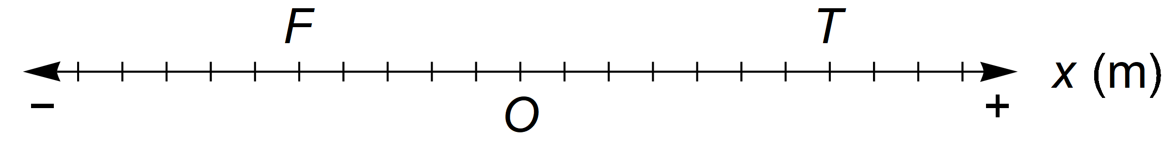
Here I’ve drawn an axis with an origin \(O\) and two objects labeled \(T\) and \(F\) at positions \(x_T = +7\,\mathrm{m}\) and \(x_F = -5\,\mathrm{m}\), respectively. We want to find the relative position of \(T\) with respect to \(F\). So, according to the procedure I described above, we can do this by placing a temporary origin \(O^F\) at the position of \(F\) and calculating \(T\)’s position along the \(x^F\)-axis.

To do this we will use the transformation equations \eqref{06122019te} and the fact that \(x_{O^F} = x_F\): \begin{equation} \begin{aligned} x_T^F &= x_T - x_{O^F} \\[1ex] &= x_T - x_F \\[1ex] &= \left( +7\,\mathrm{m} \right) - \left( -5\,\mathrm{m} \right) \\[1ex] &= +12\,\mathrm{m}. \end{aligned} \end{equation}

As always, you can count ticks to verify that the result is true. But to me, the crucial thing to notice is that because \(x_{O^F} = x_F\), we can actually cut out the whole “temporary origin” business and jump straight from \eqref{06122019te} to a new equation that gives us the relative position of any two objects \(T\) and \(F\): \begin{equation} x_T^F = x_T - x_F. \label{06122019tf} \end{equation}

Do note that the letters \(T\) and \(F\) aren’t special. They can represent any two objects, including \(A\), \(B\), \(C\), \(D\), and \(E\) from above. Or they can represent anything else. Or they can represent the same object, in which case \(x_T = x_F\) and \(x_T^F = 0\). All things are allowed, and in any case, equation \eqref{06122019tf} will provide the relative position to \(T\) from \(F\).

So do you see why I chose those letters?

“But what if we start with a different axis with a different origin? In that case, the positions of \(T\) and \(F\) will be different, too. Will they still have the same relative position between them?”

I sure hope so! Because again, the Universe doesn’t care about your origin, and something the Universe does care about like the distance between two objects shouldn’t depend upon where you set it.

Of course, you can see this from any of the axes above—no matter where you place an origin, the number of ticks and therefore distance between any two objects isn’t going to change. But let’s be algebraically sure. Given any other origin \(O’\), \eqref{06122019te} tells us that \begin{equation} \begin{aligned} x'_T &= x_T - x_{O'}, \\[1ex] x'_F &= x_F - x_{O'}. \end{aligned} \end{equation}

Then, from \eqref{06122019tf}, we find that \begin{equation} \begin{aligned} {x'}^F_T &= x'_T - x'_F \\[1ex] &= \left( x_T - x_{O'} \right) - \left( x_F - x_{O'} \right) \\[1ex] &= \left( x_T - x_F \right) + \left( x_{O'} - x_{O'} \right) \\[1ex] &= \left( x_T - x_F \right) + 0 \\[1ex] &= x^F_T. \end{aligned} \end{equation}

So, \({x’}_T^F = x_{T}^F\) for any new origin \(O’\).

\(\therefore \text{QED}\).

Alright, we’re almost at the end, but before we wrap up, there are a couple more things I would like to point out.

First, we just saw how to calculate the relative position of \(T\) with respect to \(F\). But, what if we wanted to go the other way, and find the position of \(F\) with respect to \(T\)?

We use the same formula, of course! Because again, \eqref{06122019tf} doesn’t care what the letters are: \begin{equation} x_F^T = x_F - x_T. \end{equation}

But wait a minute, that looks like something, doesn’t it?

Indeed it does: \begin{equation} \begin{aligned} x_F^T &= x_F - x_T \\[1ex] &= - \left( x_T - x_F \right) \\[1ex] &= - x_T^F. \end{aligned} \end{equation}

Therefore, for any two objects \(F\) and \(T\), \(x_T^F = - x_F^T\), which is tantamount to saying “if \(T\) is \(x\) distance to the right of \(F\), then \(F\) is \(x\) distance to the left of \(T\), and vice versa.” Obvious, right? Alas, that is why these transformations are all antisymmetric.

Finally, go way back to table \eqref{06102019xtable} and note that its real physical significance is not that it shows the positions of objects \(A\) through \(E\) along different axes centered upon objects \(A\) through \(E\) as was originally stated, but instead that it shows the relative positions of all five objects to each other, according to equation \eqref{06122019tf}. In fact, if you go even farther, you’ll see that equations \eqref{06112019ta} and \eqref{06112019tbcde}, from which we computed table \eqref{06102019xtable} and derived the transformations equations \eqref{06122019te}, are really just \eqref{06122019tf}, which is the true fundamental thing.

Thus, now, you are beginning to see the relative nature of Nature, which will lead us to interesting things.

Stay tuned,

—Aaron